
EE’s temporal analysis tools enable you to visualize the behavior of a model variable and compare it to observed data set over time. Time series plots, animations, and residual plots help you determine how concentrations change over time and how they align with your calibration targets.
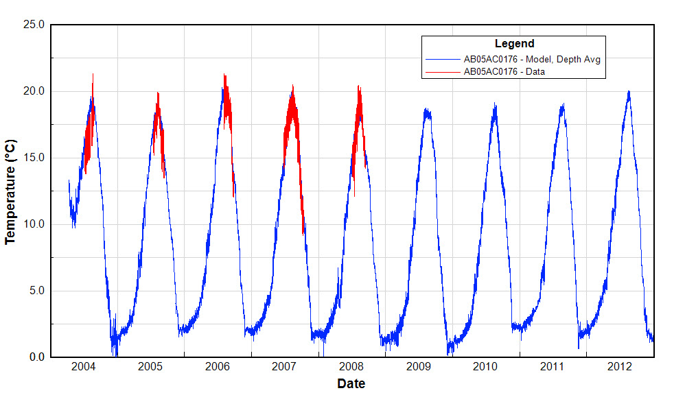
EE’s time series plots allow you to compare simulated and observed data over time and clearly illustrate historical trends.
EE has powerful 3D visualization features, including animation of slices through the X, Y, or Z plane, blanking by user-configured parameter values, flight paths, and much more.
For example, the animation to the right shows the EFDC+-simulated thermal plumes resulting from releases from a nuclear power station’s once-through cooling system.
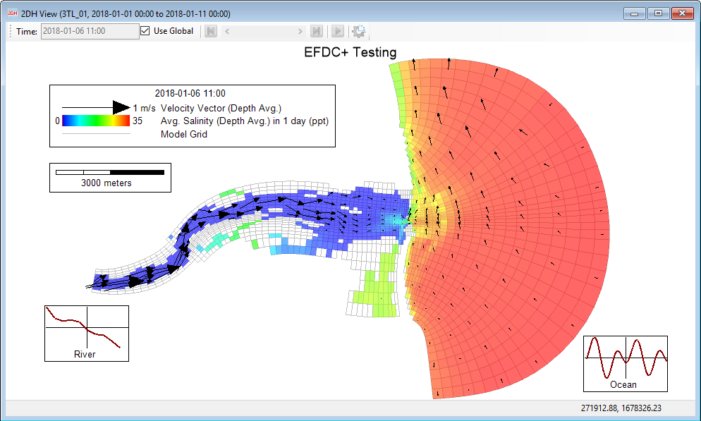
By generating residual flow fields (user-defined, time block-averaged fields), EE helps you visualize long-term model results without the “noise” of short-term impacts such as a tidal signal, for example, or other temporal boundary forcing. By removing the shorter-term impacts, you can more easily visualize and interpret the longer-term processes occurring in the waterbody. These results can also be animated.
The estuary model to the left displays a single snapshot of salinity calculated for an averaging period of a given number of hours (in this case 24 hours), with direction of flow overlaid on top.
This feature greatly aids the analysis of tidal systems.
[simpay id=”6281″]
[simpay id=”6276″]
Your support ticket has been successfully submitted. We will get back to you as soon as we can.