Vertical Layering Options in EFDC+
EFDC+ can serve as a 1-, 2-, or 3-dimensional (D) hydrodynamic model. For 3D simulations, two different vertical layering schemes are supported, allowing you to represent your system’s vertical structure appropriately. This blog will show you how to configure vertical layering and display the results in EEMS.
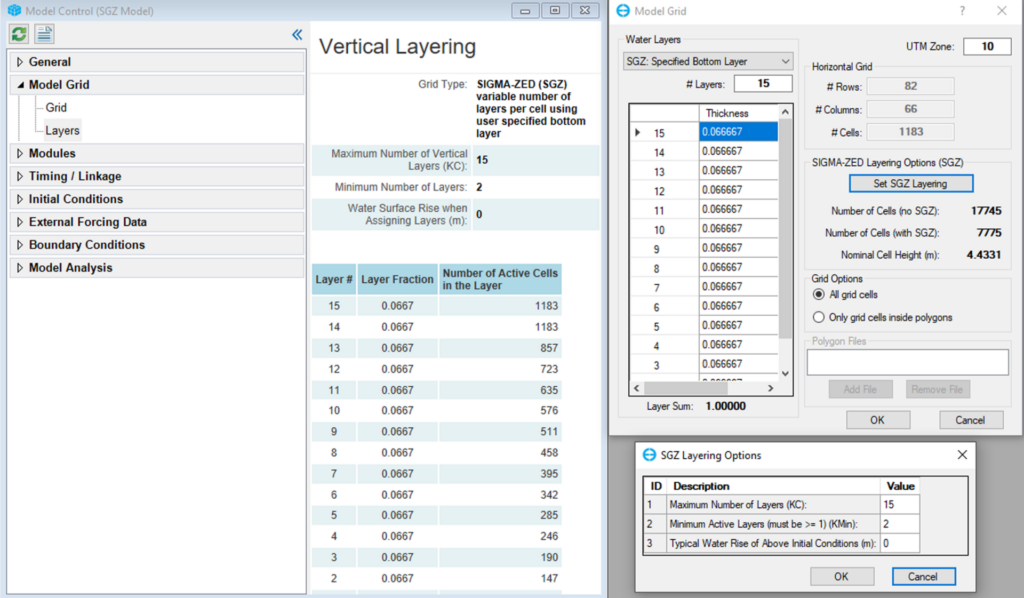
The Layers sub-menu summarizes the vertical layering in the grid. RMC on this menu item will display the options by which the user may configure the vertical layering system, as shown in Figure 1. Here, you can select the Standard Sigma grid (SIG); SGZ Variable layers, or SGZ Uniform layers. In the Water Layers form, you can set the number of layers and access a drop-down menu option for the type of layering used in the model.
The layering options are described in more detail below:
- Standard Sigma Stretch Grid: The Standard Sigma option for water layers is the original EFDC option. The traditional sigma coordinates system uses the same number of layers for all cells in the computational domain. The relative thicknesses must add up to 1 (or very close)
- Sigma-Zed Vertical Layering: The Sigma-Zed approach allows for the number of layers to vary over the model domain. Each cell can use a different number of layers, though the number of layers in that cell remains constant over time. This is computationally efficient and is now recommended as the standard approach, ensuring greatly improved accuracy.
- The specified bottom layer, the layer thickness of the adjacent cells in the vertical, does not align in the same plane. Maximum depth in the model is first calculated, and the maximum layer thicknesses are determined based on maximum depth. Zonation can be applied using this option. This is the robust option and can be applied to any type of system, such as stratified systems and systems with rapidly changing bed elevation.
The Uniform layer thickness of the cell is most of the same size as the neighboring cell. The bottom layer thickness can be 20-120% of the overlying layer. The maximum thickness is first calculated throughout the domain.
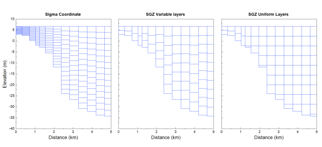
The number of grid layers and layer thickness in a transect with different water layer options is shown in Figure 2. The Sigma Coordinate option is in the left-hand panel, where all grid cells in the calculated domain are divided with the same number of layer. The middle panel is divided by the SGZ variable Layers transformation, in which the number of grid cells will be significantly reduced, and the thickness of the layers will vary uniformly based on depth. The right-hand panel is divided in a different way, with each grid cell in each layer having the same thickness, and the bottom layer having variable thickness.
Display or compare simulation results with different water layer options
To display the results in a longitudinal section, draw a centerline in 2DH View, or import from an external source. There are two ways to access 2DV View. Firstly from the main menu, select New 2DV View from the 2DV View menu item or directly click on the button from the main toolbar. You can view the results in the I, J direction or in the longitudinal section (red line), as shown in Figure 3 in the lower right panel. The remaining panels shown the temperature simulation results displayed following this vertical section with different water layer options.
Figure 4 shows the vertical profile plot comparisons between model versus observed data in three water layer cases.
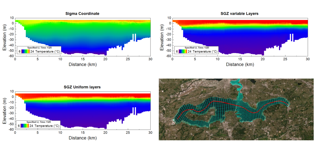
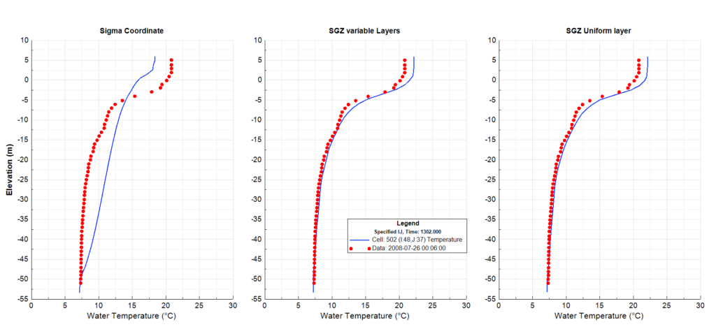
Figure 3 shows that the vertical temperature stratification using the Sigma Coordinate option is relatively poor. Similarly, Figure 4 shows that the temperature distribution under this option is almost a straight line. The SGZ option gives much better results. In addition, the total number of water column computational cells that need to be calculated when using SGZ is significantly reduced compared to Sigma Stretch, so model running time is significantly reduced.